|
Scientific Paper / Artículo Científico |
|
|
|
|
https://doi.org/10.17163/ings.n31.2024.10 |
|
|
|
pISSN: 1390-650X / eISSN: 1390-860X |
|
|
INCIDENCE OF AUTOMOTIVE AIR CONDITIONING ON THE INDEX OF FUEL CONSUMPTION IN SPARK IGNITION VEHICLE ON A ROUTE IN THE ECUADORIAN AMAZON |
||
|
INCIDENCIA DEL AIRE ACONDICIONADO AUTOMOTRIZ EN EL ÍNDICE DE CONSUMO DE COMBUSTIBLE EN VEHÍCULO DE ENCENDIDO PROVOCADO EN UNA RUTA DE LA AMAZONÍA ECUATORIANA |
||
|
Edilberto
Antonio Llanes-Cedeño1,* Vinicio
Molina-Osejos1 |
|
Received: 24-01-2023, Received after review: 07-12-2023, Accepted: 11-12-2023, Published: 01-01-2024 |
|
Abstract |
Resumen |
|
In recent years the environment has been affected by pollution produced by vehicles. The objective of this research project was to determine the incidence of air conditioning (A/C) in the vehicular fuel consumption index in the Shushufindi canton, through real traffic tests, Efficient driving mode and the use of Extra and Super gasoline, for the selection of the best alternative. The study was carried out on a route with a greater flow of vehicles, especially during normal (9:00 am) and beak (5:00 pm) hours, which comprises 16.17 km; for which used gasoline Extra (85 octane) and Super (92 octane). Data collection was carried out using an OBD2 ELM 327 system. The results obtained in the characterization of the representative mixed cycle at 9:00 am, a maximum speed of 81 km/h and an average speed of 39 km/h were obtained in a time of 1446 s route; while the mixed cycle at 5:00 pm the maximum speed is 70 km/h and an average speed of 37 km/h with a travel time of 1632 s. The lowest fuel consumption index was evidenced in normal hours, without A/C and Extra fuel (T3) with values between 0.0584 - 0.060 (L/km), and in normal hours, without A/C and super fuel (T7) that are between 0.0561-0.0585 (L/km). |
En los últimos años, el ambiente se ha visto afectado a causa de la contaminación producida por los vehículos. El presente proyecto de investigación tuvo como objetivo determinar la incidencia del aire acondicionado (A/C) en el índice de consumo de combustible vehicular en el cantón Shushufindi, por medio de pruebas reales de tráfico, modo de conducción eficiente y empleo de gasolina extra y súper, para la selección de la mejor alternativa. El estudio se realizó en una ruta de mayor flujo de vehículos, especialmente en la hora normal (9 a. m.) y pico (5 p. m.) que comprende 16.17 km, para ello se utilizó el combustible Extra (85 octanos) y Súper (92 octanos). La toma de datos se ejecutó mediante un sistema OBD2 ELM 327. Los resultados obtenidos en la caracterización del ciclo mixto representativo de 9 a. m. se obtuvo una velocidad máxima de 81 km/h y una velocidad media de 39 km/h en un tiempo de recorrido de 1446 s; mientras que el ciclo mixto de 5 p. m. la velocidad máxima es de 70 km/h y una velocidad media de 37 km/h con un tiempo de recorrido de 1632 s. El menor índice de consumo de combustible se evidenció en el horario normal, sin A/C y combustible extra (T3) siendo sus valores entre 0.0584 – 0.060 (L/km), y en el horario normal, sin A/C y combustible súper (T7) que se encuentran entre 0.0561-0.0585 (L/km). |
|
Keywords: fuel consumption index, air conditioning, efficient driving, fuel, schedule, driving cycle |
Palabras clave: índice de consumo de combustible, aire acondicionado, conducción eficiente, combustible, horario, ciclo de conducción |
|
1,*Grupo de Investigación Eficiencia, Impacto Ambiental e Innovación en la Industria y el Transporte, Facultad de Ingeniería y Ciencias Aplicadas, Carrera de Ingeniería Automotriz, Universidad Internacional SEK, Quito-Ecuador. Corresponding author ✉: antonio.llanes@uisek.edu.ec. 2Grupo de Investigación INVELECTRO, Facultad de Mecánica, Carrera de Ingeniería Automotriz, Escuela SuperiorPolitécnica de Chimborazo, Riobamba, Ecuador.
Suggested citation: Llanes-Cedeño, E.A.; Grefa Shiguango, S.F.; Molina-Osejos, J.V. and Rocha-Hoyos, J.C. “Incidence of automotive air conditioning on the index of fuel consumption in spark ignition vehicle on a route in the ecuadorian amazon,” Ingenius, Revista de Ciencia y Tecnología, N.◦ 31, pp. 115-126, 2024, doi: https://doi.org/10.17163/ings.n31.2024.10. |
|
1. Introduction
According to AEADE [1], in Ecuador, an annual sale of 132,000 vehicles is recorded, representing a high sales rate in the market that varies according to the country’s economic situation. However, the number of cars directly influences environmental pollution. For this reason, Ecuador has adopted Euro 3 regulations to control pollution. Nevertheless, due to the poor fuel quality, the pollution index of vehicles has directly impacted the environment. Air pollution is one of the most severe global environmental issues today. Gas emissions are linked to the hydrocarbons found in the fuel used for vehicles. These vehicular emissions manifest through the combustion of hydrocarbons (HC), nitrogen oxides (NOx), carbon monoxide (CO), and carbon dioxide (CO2), directly impacting the public health of the country [2]. Climate change has been observable for many years, increasingly evoking heightened concern. The greenhouse gas emissions produced have intensified vulnerability in the natural regions of Ecuador [3]. Según Guzmán et al. [4] and Llanes et al. [2] assert that Super gasoline produces low emissions and relatively lower fuel consumption than Extra gasoline. Ecopaís fuel was introduced in Guayaquil in 2010 as the primary choice for consumers due to its costeffectiveness compared to other fuels [5]. Initially proposed with an octane rating of 80, it has recently been regulated between 85 and 87 octane. In contrast to Extra gasoline, it contains 5% ethanol, derived from corn and sugarcane. At present, there is considerable interest in driving cycles, represented by driving patterns and utilized to comprehend energy consumption, fuel consumption, and exhaust gas emissions in vehicles [6]. According to Tong & Hung [7], the driving cycle is a time series of speeds that describes the driving pattern; thus, the driving pattern plays a crucial role in a driving cycle. In 1960, the Federal Test Procedure (FTP) cycle was conducted through a conventional driving route in Los Angeles, California. Established parameters included vehicle speed, engine speed, and intake manifold pressure. A 1964 Chevrolet was used for the 12-mile route. In 2002, Ecuador adopted the FTP 75 test cycle following the NTE INEN 2204 standard, designed for light and medium vehicles using gasoline [8]. The New European Driving Cycle (NEDC) is used for homologating vehicles that comply with Euro 6 regulations in Europe and other countries. Commonly referred to as ECE for urban areas, repeated four times, and EUDC for extra-urban regions, it serves as a standardized procedure. According to Romain [9], the main characteristics of the cycle are distance: 11,023 m, duration: 1180 s, and an average speed: 33.6 km/h. |
The European cycle has been criticized for not accurately representing real driving conditions in recent years. It features very smooth accelerations, constantspeed cruising, and periods of inactivity, posing a challenge in obtaining a certificate that genuinely reflects the vehicle’s performance in real-world conditions [9]. Wang et al. [10] mention the use of specially designed instruments for recording speed and travel time, incorporating a GPS and a speed sensor to monitor data quality. Conversely, Morey, Limanond, & Niemeier [11] emphasize that overrepresenting driving data during peak hours compared to non-peak hours may compromise their representativeness of real driving conditions. Hence, they highlight the significance of conducting route tests during peak hours, as they yield valid data corresponding to the specific situation of the city or study area. The analysis of driving patterns proposed by Joumard et al. [12] covers speed, acceleration, and braking rates, ranging from highly congested urban driving to highway conditions. The research results reveal variations between 10% and 20% in pollutant emissions in urban areas, with rural emissions experiencing a slight decrease. According to Urbina et al. [13], the On-Board cycle enables on-road tests under real traffic conditions, measuring emission concentrations, fuel consumption, and distance traveled. To achievethis, a mixed cycle in city and highway settings was utilized, demonstrating lower CO emission factors than the IM240 cycle. Jiménez, Román & López [14] highlight global parameters influencing driving dynamics, including maximum speed (km/h), average speed (km/h), average acceleration (m/s2), average deceleration (m/s2), duration (s), among others. The selection of driving patterns depends on the vehicle, terrain, traffic data, and other factors, underscoring the importance of defining routes that represent typical driving patterns to gather relevant data for the vehicle study. Ternz & Ternz [15] and Huang et al. [16] mention the following list of techniques associated with ecofriendly driving: (1) moderate acceleration with shifts between 2000-2500 revolutions for manual transmissions; (2) anticipate traffic flow and signals, avoiding constant starts and stops; (3) maintain a constant speed; (4) avoid high speeds; (5) vehicle maintenance according to the manufacturer’s manual; (6) turn off the engine during prolonged stops; (7) maintain optimal tire pressure and regularly change the air filter. According to Barkenbus [17], eco-friendly driving reduces fuel consumption by an average of 10%, thereby gradually lowering CO2 emissions from driving by an equivalent percentage. Additionally, Mensing et al. [18] found that emissions and fuel consumption increase due |
|
to the extended time spent in high-acceleration engine operation. The air conditioning (A/C) system in cars has enhanced people’s comfort and, to some extent, their safety when driving in adverse weather conditions [19]. However, using A/C results in energy loss and an increase in fuel consumption and polluting gas emissions [20]. In the study conducted in the highland and coastal regions, Acosta & Tello [21] state that the thermal comfort in the cabin ranges between 22 and 27 ºC, with a relative humidity between 45% and 65%. In contrast, Pérez & Córdova [22] mention that, for the coastal region, the comfortable temperature ranges between 20 and 24 ºC, attributed to the climate characteristic of cities located at sea level. The A/C has the most significant impact on fuel consumption. Tamura, Yakumaru, & Nishiwaki [23] reported additional fuel consumption ranging between 2.5% and 7.5% due to the performance of the air conditioning, considering factors such as climatic conditions, engine type, and user profile. It is known that the use of air conditioning affects emission factors and the fuel consumption index in driving conditions in the Amazonian regions. However, there is insufficient information available regarding the driving cycle. Therefore, this study aimed to assess the incidence of air conditioning on the vehicular fuel consumption index in the Shushufindi canton through accurate traffic tests, implementing Eco driving mode and using Extra and Super gasoline to choose the best alternative.
2. Materials and methods
The study adopts a quantitative approach, focusing on characterizing a specific route to evaluate the fuel consumption index in the Ecuadorian Amazon region through experimental calculations and statistical operations. The research can be classified as exploratory and field-based, involving the review of various types of studies and the execution of an on-board driving cycle on a real route that spans urban and rural environments, including roads.
2.1.Study area
The Shushufindi canton, situated in the province of Sucumbíos in the Amazon Region of Ecuador, was selected, as illustrated in Figure 1 (marked with a red point). This location sits at an elevation of 240 meters above sea level and shares borders with the cantons of Lago Agrio and Cuyabeno to the north, the province of Orellana to the south and west, and the canton of Cuyabeno to the east. The ambient temperature in this area ranges between 26 and 30 ºC. |
Figure 1. Map of the study area. Shushufindi Canton (Google Maps [24])
2.2.Route characterization
For the selection of the route, various criteria were taken into account. These criteria included roads with higher traffic flow, slow acceleration lanes, free acceleration lanes, and the type of road [12]. The altitude and coordinate data for the study were obtained using a GPSMAP 62s. The information collection was conducted directly with the vehicle. The stored data was then filtered in Excel to perform statistical analysis and obtain the driving cycle. Figure 2 displays the points obtained through Google Earth, covering a route that includes urban and rural environments (roads).
Figure 2. Established urban-rural route. Shushufindi Canton
This study encompasses a route of 16.17 km that includes the urban area with streets and avenues with heavy traffic, such as Perimetral Avenue, Policía Nacional Avenue, Unidad Nacional Avenue, Aguarico 3 Avenue, 11 de Julio Avenue, Napo Avenue, Siona Street, Oriental Street, and Naciones Unidas Avenue. On the other hand, the rural part of the route includes the Shushufindi-Limoncocha Road and San Mateo Avenue. According to Safety Enforcement Seguridad Vial S. A. [25], speed limits for light vehicles in urban areas are 50 km/h, with a maximum of 60 km/h. The speed range for straight sections on the road is from 100 to 135 km/h, while for curves on the road, the speed is 60 km/h, with a maximum of 75 km/h. The ELM 327 (OBD2) device was used to obtain speed, acceleration, and time data.
|


|
Based on the proposals of Tong & Hung [7] and Quinchimbla & Solís [26], the following parameters are deduced for this study: distance traveled (km), maximum speed (km/h), average speed (km/h), travel time (s), average positive acceleration (m/s2), time with positive acceleration (s), and, finally, the number of stops. The driving cycle was established through weightings. Gómez [27] developed the driving cycle for the central-western metropolitan area in Colombia, determined by weighted parameters. Valdez [28] developed vehicle driving cycles in Naucalpan, Mexico City, and the United States, among other locations. This is represented by the result of a sample of experimental curves obtained by comparing the most influential variables of each experiment. The variables are identified based on their relevance to each parameter. The weighting is set on a scale from 0 to 1, and the value of each parameter is composed of multiples of 0.25 [28,29]. Table 1 displays the weighting assigned to each previously established parameter.
Table 1. Weighting table for each parameter
Equation (1) considers the
smaller value Y, representing a lesser deviation from the mean. In this equation,
Y corresponds to the weighted average, Wi is the weighting coefficient for
each average, Pi,j is the parameter value,
2.3.Test vehicle. Fuels
For this study, the chosen vehicle is the BEAT PREMIER AC 1.2 4P 4X2 TM, as depicted in Figure 3. According to the Association of Automotive Companies of Ecuador, this vehicle was among the top-selling models in 2019, with over 4,125 units sold, and its commercial availability extends through 2021. This car is recognized |
for its comfort, safety features, stylish design, and advanced technology. Additionally, it is noteworthy for its low fuel consumption and spare parts utilization [30]. In the Amazon region, it is one of the most in-demand vehicles due to its cost-effectiveness and accessibility.
Figure 3. Chevrolet BEAT
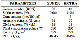
In the chosen test, the vehicle underwent preventative maintenance, encompassing the ABC of the engine (oil changes, air filter, and fuel filter). Additionally, the proper functioning of the electronic injection system was verified, and an electronic examination was conducted using a scanner. Likewise, the tire pressure was ensured to align with the manufacturer’s specifications, set at 30 PSI of air in each tire. These procedures validated the correct vehicle operation for the respective study test. The fuel consumption (Extra and Super) on the established route was determined using the OBD2 ELM327. According to Cortez and Alejandro [31], the OBD2 is an electronic device capable of automatically identifying the communication protocol of the ECU and enables the reading and clearing of codes. The “Car Scanner ELM OBD2” application was used for data collection, allowing the user to read and record real-time operating data of the car’s variables. Additionally, it facilitates the wireless transmission of ECU information to the mobile phone using Bluetooth technology. Table 2 displays the primary characteristics of the utilized fuels.
Table 2. Fuel properties. Note: Taken from the study conducted by Taipe-Defaz et al. [32]
|


|
Figure 4 illustrates the air conditioning system’s components [21]; the refrigerant employed is R-134a.
Figure 4. Automotive air conditioning components
2.4.Efficient driving protocol
Efficient driving requires the driver to adhere to a set of parameters while operating the vehicle. The guidelines, as proposed by Ternz and Ternz [15] and Mensing et al. [18], are as follows: (1) execute gear changes between 2000 and 2500 rpm, (2) utilize the first gear solely to initiate vehicle movement, (3) apply smooth acceleration without excessive pedal pressure, (4) shift to second gear at the earliest opportunity, (5) capitalize on the vehicle’s gravity and inertia when descending slopes (avoid fully depressing the accelerator), (6) anticipate traffic to minimize frequent starts and stops, (7) prioritize braking using the engine brake, (8) when using air conditioning on routes, keep all windows completely closed; for routes without A/C, keep the windows down, (9) avoid sudden braking and acceleration, (10) maintain a consistent speed (80 km/h-90 km/h maximum in perimeter areas and 45 km/h in urban areas), (11) refrain from high speeds on highways and urban routes, (12) consistently attempt to use the highest possible gear, and (13) ultimately, turn off the engine during prolonged stops.
2.5.Experimental Design
A factorial multilevel design was created to evaluate the fuel consumption index using STATGRAPHICS Centurion XVI software. For this purpose, the factors of fuel, air conditioning, and schedule were established, each represented by two levels, as detailed in Table 3. |
Table 3. Design of the factors and levels to be considered
Table 4 displays the response variables: Fuel consumption index (L/km) of the experimental design.
Table 4. Response variables of the experimental design
The Statgraphics Centurión XVI software was used to analyse and compare the results. A simple ANOVA was conducted for the different treatments (combinations) detailed in Table 5. In this analysis, the Fisher’s Least Significant Difference (LSD) procedure was applied with a confidence level of 95.0%. Three repetitions were carried out for each treatment, following the guidelines of the NTE INEN 2205 standard in Section 6 on test methods. Section 6.1.5.4 specifies: "Record and average a minimum of 3 readings for each test" (24 tests were conducted) [33].
Table 5. Treatment for response surface analysis
2.6.Test protocol
A driver was chosen to carry out 24 route tests. This driver was provided with information about the efficient driving pattern and the route to follow, considering the recommendations of Milla, Cedeño and Hoyos [34]. |


|
The proposed route covers 16.17 kilometers and is conducted under the following conditions: (1) two initial scenarios are considered for the test, one during regular hours (9 a.m.) and another during peak hours (5:00 p.m.); (2) tests are performed using two types of fuel (Extra and Super). For the test with Extra fuel, the vehicle’s fuel tank is filled completely at the beginning and end of the route. The same procedure is applied for the test with Super fuel; (3) the OBD2 connector is connected to the ELM 327 measurement equipment (Figure 5); (4) the Car Scanner ELM OBD2 application is activated to record information on fuel consumption, speed, acceleration, and time; (5) the test is initiated after verifying the proper connection of all equipment; (6) the established route is followed until completion with the same driver; (7) upon completing the route, the information is saved in a file and exported to Excel software for analysis and tabulation of results. These steps are repeated for treatments according to the established levels: regular hours, peak hours, with A/C, without A/C, Extra fuel, and Super fuel.
Figure 5. OBD2 ELM 327 Mini Module and Car Scanner Application
3. Results and discussion
This section presents the results obtained by executing tests at different times (regular and peak hours) on a predetermined route, as detailed in the methodology. The weighting formula was applied to determine the estimated results of route characterization, selecting the value with the least variability and the result that most accurately represents the collected data.
3.1.Mixed cycle. Regular hours (9 a.m.)
The first established route was carried out during regular hours with less traffic congestion. In this case, three complete trips were conducted. The values were obtained through everyday driving with a weighting of Y = 0.0316. Figure 6 illustrates that the maximum speed reached 81 km/h, with an average speed of 39 km/h over a travel time of 1446 s (24.1 min). Throughout the journey, 4 stops were made, with an average positive acceleration of 0.479 m/s2 |
and a positive acceleration time of 520 s. Additionally, there is evidence of speed variability corresponding to rural and urban routes. In the study conducted by Pérez y Quito [29], a weighted mean of Y = 0.097 was recorded in a combined cycle conducted in Cuenca, demonstrating less deviation in the proposed results, with a 31% lower variability compared to the study. Table 6 presents the values corresponding to the driving cycle.
Figure 6. Graph illustrating data during regular hours
Table 6. Characteristic parameters corresponding to regular hours (9 a.m.)
3.2.Mixed cycle. Peak hours (5 p.m.)
Figure 7 depicts the peak hours with increased vehicular traffic, primarily due to the presence of businesses and factories along the route. The lowest weighted mean of Y = 0.0241 was obtained. The values were determined through everyday driving. Figure 7 illustrates that the maximum speed reached 70 km/h, with an average speed of 37 km/h over a travel time of 1632 s (27.2 min). Throughout the journey, 5 stops were made, with an average positive acceleration of 0.427 m/s2 and a positive acceleration time of 452 s. Additionally, there is evidence of speed variability corresponding to the urban area, reaching a speed of 48 km/h. The cycle proposed by Quinchimbla y Solís [26] records a weighted mean of Y = 0.1168 in a combined route conducted in Quito, exhibiting a 9% variability compared to the proposed study and a maximum 72 km/h speed. This demonstrates an acceptable correlation with the proposed cycle. Table 7 presents the parameters corresponding to the representative peak hours. |


|
Figure 7. Graph illustrating data during peak hours
Table 7. Characteristic parameters corresponding to peak hours (5 p. m.).
3.3. Comparison between Regular Hours and Peak Hours
Figure 8 shows the representative cycle corresponding to the journey during regular and peak hours, with a weighted mean value of Y = 0.0316 at 9 a.m. and Y = 0.0241 at 5 p.m.
Figure 8. Comparative graph of representative mixed cycles
It can be observed that the maximum speed is 81 km/h during regular hours and 70 km/h during peak hours. Additionally, speed variability in urban and rural areas is attributed to vehicular congestion within the allowed limits for each sector. For example, the average speed was 39 km/h during regular hours, whereas it was 34 km/h during peak hours. Similarly, the travel time during regular hours was 1446 s, whereas during peak hours, it was 1632 s. Thus, it is evident that the highest congestion occurs on the urban route, particularly during peak hours due to traffic lights and vehicle stops. The findings align with the study conducted by Quinchimbla y Solís [26], |
where the distance covered in combined cycles from various research was compared, resulting in an average distance of 15973.75 m. Given that the proposed study covers 1600.17 m, it is validated to fall within the allowed limits. Additionally, the driving parameters of the combined cycle are compared with various studies, determining that the cycle is highly variable due to geographical conditions, traffic density, and road infrastructure, which can influence the obtained driving parameters. Therefore, the obtained values vary compared to European, American, or other cycles.
3.4.Fuel consumption index
The fuel consumption index (FCI) was calculated following the test protocols mentioned in the methods. The FCI was evaluated using the STATGRAPHICS Centurion XVI software, entering the values corresponding to the fuel consumption obtained in the tests conducted on the vehicle. Figure 9 illustrates that the factors influencing the fuel consumption index include air conditioning (A/C), fuel type, schedule, and the combination of fuel and schedule. Conversely, the BC and AB combinations do not impact fuel consumption. According to the analysis of variance for the fuel consumption index (FCI), the adjusted model accounts for 98.8% of the variability in FCI with a confidence level of 95%.
Figure 9. Standardized Pareto diagram for FC
Figure 10 shows the main effects for the fuel consumption index (FCI). When using Extra fuel (1), FCI increases. Conversely, when using Super fuel (2), FCI improves. Using air conditioning (2) significantly increases FCI, while FCI (1) without air conditioning is relatively lower. Additionally, FCI increases during peak hours (2) and decreases during regular hours. Thus, the optimal minimum value is 0.057 (L/km), obtained with the combination 2-1-1 (Super-Reg. Hours-No A/C).
|


|
Figure 10. Main effects graph for FC
Figure 11 illustrates that the fuel consumption index (FCI) is lower when A/C = 1 (no A/C); however, the time factor does not exert an impact. The influential value for fuel = 1 (Extra) is obtained when A/C is not in use, yielding an optimal value of 0.06 L/km, with time not significantly impacting. Lower values are observed during regular hours, even when time, based on observed shading, does not exert a considerable impact; nevertheless, it is evident that the most favourable results are obtained for time 1 (regular). When using fuel = 2 (Super), the lowest values are achieved when not employing air conditioning, resulting in an optimal value of 0.058 L/km, with time not significantly influencing. Lower values are obtained during regular hours, even though regular hours do not exert a significant impact, leading to the lowest results compared to peak hours. Consequently, Super fuel exhibits lower fuel consumption indices without air conditioning and under regular time conditions. This study aligns with Andrade [35], who conducted research with the Chevrolet Aveo vehicle under sea-level conditions, concluding that Super gasoline yields lower fuel consumption indices, demonstrating better mileage performance and representing a lower long-term cost. In the study conducted by García and Villalba [36], it is observed that the fuel consumption index decreases with efficient driving, achieving a fuel optimization of 28.34%; nevertheless, the proposed study is based on regular time conditions.
|
Figure 11. Estimated response surface FC. a) Extra fuel vs. b) Super gasoline
Figure 12 illustrates the behavior of the Fuel Consumption Index (FCI) concerning the type of fuel utilized and the activation of air conditioning (A/C) when the schedule is set to 1 (regular). In this context, it is observed that the lowest CI values are attained with Super fuel (2) and without A/C (1), resulting in a value of 0.058 L/km. Conversely, when the schedule is adjusted to 2 (peak), the lowest CI values are derived from Super fuel, Extra fuel, and the absence of A/C. While the fuel factor does not exert a direct influence based on the observed hue, it is perceived that Super fuel yields lower outcomes. In summary, using air conditioning during peak hours corresponds to an elevation in the fuel consumption index. These findings align with the results of a study conducted by Arias and Ludeña [37] involving the Chevrolet Aveo Activo vehicle in Cuenca. Their study concluded that fuel consumption increases during peak hours, whereas it decreases during regular hours. This implies that peak hours, characterized by heightened traffic congestion, are associated with a higher fuel consumption index irrespective of the day. |


|
Figure 12. Estimated response surface FC. a) Regular hours and b) Peak hours
Figure 13 illustrates the behavior of the Fuel Consumption Index (FCI) concerning the type of fuel used and the travel schedule. When A/C = 1 (without A/C), it is observed that the lowest CI values are achieved with Super fuel (2) during regular hours (1), reaching a value of 0.057 L/km. As the quality of the fuel increases, more favorable results are obtained in the CI, and less traffic on the route also positively influences the CI. However, the schedule and fuel type are insignificant, although lower results are noted for regular hours and Super fuel based on the observed hue. When A/C = 2 (with A/C), it is observed that the lowest CI values are obtained with fuel type 2 (Super) during schedule 1 (regular), signifying that the lowest CI values are attained with higher-quality fuel. As the fuel quality improves, the CI results also show improvement, and the traffic reduction on the route positively impacts the CI. The study conducted by Chancafe [38] confirms that using air conditioning increases vehicle fuel consumption. According to Acosta & Tello [21], the highest fuel consumption rates were recorded on the road using air conditioning. It is noteworthy that as one descends to lower altitudes, consumption increases due to the correction made for the higher levels of oxygen present. |
Figure 13. Estimated response surface FC. a) Regular hours and b) Peak hours
Figure 14 illustrates the box and whisker plot of the fuel consumption index. It is observed that treatments T7 (Super-without AC-H. regular) and T3 (Extrawithout AC-H. regular) fall within the range of 0.057 to 0.073 L/km, with T7 exhibiting the least significant difference. This is attributed to the use of Super fuel, which has an octane rating of 92, promoting engine combustion. Furthermore, the absence of air conditioning (A/C) reduces the fuel consumption index (FCI). Treatment T3 also complies with the permitted usage limits, indicating that both T3 and T7 exhibit optimal responses. Conversely, treatments T1, T2, T4, T5, T6, and T8 demonstrate elevated fuel consumption indices.
Figure 14. FC Box and whisker graph |


|
Table 8 presents the results obtained from applying the LSD (Fisher) test with a 95% confidence level. It is evident that in treatments T7 (Super-Without A/C-Regular Schedule) and T3 (Extra-Without A/CRegular Schedule), no significant differences are observed. These findings align with the conclusions of Andrade [35], who asserts that the use of Super gasoline is associated with lower fuel consumption indices. Additionally, Arias and Ludeña [37] determine that the fuel consumption index tends to be lower during regular schedules. Chancafe [38] confirms that the absence of air conditioning results in lower fuel consumption indices. Therefore, it is suggested that the most suitable treatment for the Amazon region is T7, with an average efficiency of 17.45 km/L. However, due to the cost of Super gasoline, it is recommended to use treatment T3, which provides an efficiency of 16.86 km/L. This treatment includes Extra fuel, no A/C, and a regular schedule, as it does not exhibit significant differences. It is crucial to adopt efficient driving practices since, under normal conditions, the impact on fuel consumption significantly increases. In contrast, treatments T1, T2, T4, T5, T6, and T8 exhibit significant differences, emphasizing peak hour factors and A/C usage, resulting in an increased fuel consumption index.
Table 8. Multiple range tests
4. Conclusions
The statistical method, chosen by applying weighting criteria on each established route, facilitated the identification of representative journeys characterized by minimal deviations from the average. During regular hours, a Y value of 0.0316 was obtained, while during peak hours, a Y value of 0.0241 was achieved, indicating a 31% reduction compared to the literature under investigation. In regular hours (9 a.m.), the recorded data included a maximum speed of 81 km/h and an average speed of 39 km/h, with a travel time of 1446 s (24.1 minutes). Conversely, during peak hours (5 p.m.), the maximum speed reached 70 km/h, with an average speed of 37 km/h and a travel time of 1632 s (27.2 minutes), resulting in a 10% difference. |
The road test conducted with the Chevrolet Beat vehicle determined that the optimal lowest value of the fuel consumption index (FCI) is attained during regular hours, without A/C, and using Super fuel. Consequently, it is concluded that the significant factors influencing the FCI include the use of air conditioning (A/C), Extra gasoline, and peak hours in the Shushufindi canton, situated in the Eastern region of Ecuador. In the study of the fuel consumption index (FCI), it was determined through the LSD test with a 95% confidence level that treatment T3 (regular schedule, without A/C and Extra fuel), with values ranging from 0.0584 to 0.060 L/km and treatment T7 (regular schedule, without A/C, and Super fuel), with values between 0.0561 and 0.0585 L/km, demonstrate optimal savings in the fuel consumption index when applying efficient driving practices. Further research encompassing various vehicles, brands, and models is recommended. This will facilitate a comprehensive understanding of the dynamics associated with fuel, air conditioning, and regular and peak schedules.
References
[1] AEADE, Anuario 2019. Asociación de Empresas Automotrices del Ecuador, 2019. [Online]. Available: https://bit.ly/3Rl41yA [2] E. A. Llanes Cedeño, J. C. Rocha-Hoyos, D. B. Peralta Zurita, and J. C. Leguísamo Milla, “Evaluation of gas emissions in light gasoline vehicles in height conditions. case study quito, ecuador,” Enfoque UTE, vol. 9, no. 2, pp. 149–158, Jun. 2018. [Online]. Available: https://doi.org/10.29019/enfoqueute.v9n2.201 [3] FLACSO, GEO Ecuador 2008 Informe sobre el estado del arte del medio ambiente. FLACSO, MAE, PNUMA, 2008. [Online]. Available: https://bit.ly/4aC6v4K [4] A. R. Guzmán, E. Cueva, A. Peralvo, M. Revelo, and A. Armas, “Study of the dynamic performance of an otto engine using mixtures two types of extra and super gasolines,” Enfoque UTE, vol. 9, no. 4, pp. 208–220, Dec. 2018. [Online]. Available: https://doi.org/10.29019/enfoqueute.v9n4.335 [5] D. G. Perez Darquea, “Estudio de emisiones contaminantes utilizando combustibles locales,” INNOVA, vol. 3, no. 3, pp. 23–34, 2018. [Online]. Available: https://doi.org/10.33890/innova.v3.n3.2018.635
|

|
[6] L. F. Quirama, M. Giraldo, J. I. Huertas, and M. Jaller, “Driving cycles that reproduce driving patterns, energy consumptions and tailpipe emissions,” Transportation Research Part D: Transport and Environment, vol. 82, p. 102294, 2020. [Online]. Available: https://doi.org/10.1016/j.trd.2020.102294 [7] H. Y. Tong and W. T. Hung, “A framework for developing driving cycles with on-road driving data,” Transport Reviews, vol. 30, no. 5, pp. 589–615, 2010. [Online]. Available: https://doi.org/10.1080/01441640903286134 [8] INEN, NTE INEN 2204 Gestión ambiental. Aire. Vehículos automotores. Límites permitidos de emisiones producidas por fuentes móviles terrestres que emplean gasolina. Instituto Ecuatoriano de Normalización, 2017. [Online]. Available: https://bit.ly/3ROTgpG [9] N. Romain. (2013) The different driving cycles. Car Engineer. Car Engineer. [Online]. Available: https://bit.ly/3RrVZ7e [10] Q. Wang, H. Huo, K. He, Z. Yao, and Q. Zhang, “Characterization of vehicle driving patterns and development of driving cycles in chinese cities,” Transportation Research Part D: Transport and Environment, vol. 13, no. 5, pp. 289–297, 2008. [Online]. Available: https://doi.org/10.1016/j.trd.2008.03.003 [11] J. E. Morey, T. Limanond, and D. A. Niemeier, “Validity of chase car data used in developing emissions cycles,” Statistical Analysis and Modeling of Automotive Emissions, vol. 3, no. 2, pp. 15–28, Sep 2000, journal Article. [Online]. Available: https://bit.ly/3RN5wXO [12] M. André, R. Joumard, R. Vidon, P. Tassel, and P. Perret, “Real-world european driving cycles, for measuring pollutant emissions from high- and low-powered cars,” Atmospheric Environment, vol. 40, no. 31, pp. 5944–5953, 2006, 13th International Symposium on Transport and Air Pollution (TAP-2004). [Online]. Available: https://doi.org/10.1016/j.atmosenv.2005.12.057 [13] A. Urbina, L. Tipanluisa, and A. Portilla, “Estudio de las emisiones vehiculares en pruebas con dinamómetro y en ruta,” in VIII Congreso Internacional de Ingeniería Mecánica y Mecatrónica, 04 2017. [Online]. Available: https://bit.ly/41prHGZ [14] F. Jiménez Alonso, A. Román, and J. M. López Martínez, “Determinación de ciclos de conducción en rutas urbanas fijas,” DINA Ingeniería e Industria, vol. 88, pp. 681–688, 2013. [Online]. Available: https://doi.org/10.6036/5751 [15] R. Luther and P. Baas, Eco-Driving Scoping Study. Energy Efficiency and Conservation Authority, 2011. [Online]. Available: https://bit.ly/41wjq3T |
[16] Y. Huang, E. C. Ng, J. L. Zhou, N. C. Surawski, E. F. Chan, and G. Hong, “Eco-driving technology for sustainable road transport: A review,” Renewable and Sustainable Energy Reviews, vol. 93, pp. 596–609, 2018. [Online]. Available https://doi.org/10.1016/j.rser.2018.05.030 [17] J. N. Barkenbus, “Eco-driving: An overlooked climate change initiative,” Energy Policy, vol. 38, no. 2, pp. 762–769, 2010. [Online]. Available: https://doi.org/10.1016/j.enpol.2009.10.021 [18] F. Mensing, E. Bideaux, R. Trigui, J. Ribet, and B. Jeanneret, “Eco-driving: Aneconomic or ecologic driving style?” TransportationResearch Part C: Emerging Technologies,vol. 38, pp. 110–121, 2014. [Online]. Available: https://doi.org/10.1016/j.trc.2013.10.013 [19] B. A. Cuaical Angulo and E. Torres Tamayo, “Caracterización de la eficiencia energética en los sistemas de refrigeración aplicados en el área automotriz,” INVPOS, vol. 1, no. 1, pp. 1–16, 2018. [Online]. Available: https://bit.ly/41qG3H7 [20] M. d. J. Guananga Totoy, Díseño y construcción de un simulador de climatización automotriz. Universidad Internacional del Ecuador, 2013. [Online]. Available: https://bit.ly/3TrvRfr [21] M. A. Acosta Corral and W. P. Tello Flores, Estudio del aire acondicionado en el consumo de combustible, potencia del motor y confort térmico en la cabina de un vehículo liviano. Escuela Politécnica Nacional, 2016. [Online]. Available: https://bit.ly/3NBhuBw [22] M. A. Córdova Suárez and C. F. Pérez Salinas, El gasto metabólico y la temperatura WBGTt en el sistema de trabajo de conductor de bus tipo volkswagen 17210 de la carrocería Modelo Orión Marca Imce y su incidencia en el estrés térmico. Universidad Técnica de Ambato, 2014. [Online]. Available: https://bit.ly/3RmP3bm [23] T. Tamura, Y. Yakumaru, and F. Nishiwaki, “Experimental study on automotive cooling and heating air conditioning system using CO2 as a refrigerant,” International Journa of Refrigeration, vol. 28, no. 8, pp. 1302–1307, 2005, cO2 as Working Fluid -Theory and Applications. [Online]. Available: https://doi.org/10.1016/j.ijrefrig.2005.09.010 [24] Google. (2023) Shushufindi. Google Maps. Google Maps. [Online]. Available: https://bit.ly/475PMDF [25] SES. (2018) Los limites de velocidad en el Ecuador. Safety Enforcement Seguridad Vial S.A. (SES). Safety Enforcement Seguridad Vial S.A. (SES). [Online]. Available: https://bit.ly/3RPAiyn [26] F. E. Quinchimbla Pisuña and J. M. Solís Santamaría, Desarrollo de ciclos de conducción en ciudad, carretera y combinado para evaluar el rendimiento real del combustible de un vehículo con motor de ciclo Otto en el Distrito Metropolitano de Quito. Escuela Politécnica Nacional 2017. [Online]. Available: https://bit.ly/3TrKtvi |
|
[27] A. Hurtado Gómez, Desarrollo de ciclos de conducción para el área metropolitana Centro Occidente-AMCO. Universidd Tecnológica de Pereira, 2014. [Online]. Available: https://bit.ly/41thLvY [28] A. Valdéz Aguilera, Desarrollo de Ciclos de Conducción Vehicular en el Municipio de Naucalpan. Tecnológico de Monterrey, 2004. [Online]. Available: https://bit.ly/3RQEDSM [29] P. S. Pérez Llanos and C. O. Quito Sinchi, Determinación de los ciclos de conducción de un vehículo categoría M1 para la ciudad de Cuenca. Universidd Politécnica Salesiana, 2018. [Online]. Available: https://bit.ly/3ROiIf0 [30] Chevrolet, Datasheet Chevrolet Beat 2021. Chevrolet Ecuador, 2021. [Online]. Available: https://bit.ly/4aqb6H0 [31] M. A. Pinto Cortez, Investigación de los parámetros característicos de desempeño del motor de combustión interna efi al utilizar la interfase ECOOBD2. Universidad de las Fuerzas Armadas, 2019. [Online]. Available: https://bit.ly/3v8TgZ1 [32] V. A. Taipe-Defaz, E. A. Llanes Cedeño, C. F. Morales-Bayetero, and A. E. Checa-Ramírez, “Evaluación experimental de un motor de encendido provocado bajo diferentes gasolinas,” Ingenius, no. 26, pp. 17–29, 2021. [Online]. Available: https://doi.org/10.17163/ings.n26.2021.02 [33] INEN, NTE INEN 2205:2010, Vehículos Automotores. Bus Urbano. Requisitos. Instituto Ecuatoriano de Normalización, 2010. [Online]. Available: https://bit.ly/3TwXl36 |
[34] J. C. Leguísamo Milla, E. Llanes Cedeño, and J. Rocha Hoyos, “Impact of ecodriving on fuel emissions and consumption on road of quito,” Enfoque UTE, vol. 11, no. 1, pp. 68–83, Jan. 2020. [Online]. Available: https://doi.org/10.29019/enfoque.v11n1.500 [35] F. L. Morquecho Andrade, “Análisis de rendimiento y costo de los combustibles Ecopaís y súper,” Innova, vol. 3, no. 1, pp. 135–149, 2018. [Online]. Available: https://doi.org/10.33890/innova.v3.n10.1.2018.899 [36] N. G. García Jaramillo and J. R. Villalba Arteaga, Estudio del efecto de la conducción eficiente sobre el consumo y las emisiones. Universidad Internacional del Ecuador, 2016. [Online]. Available: https://bit.ly/3RRXTzD [37] E. I. Arias Montaño and J. A. Ludeña Ayala, Estimación del consumo de combustible y niveles de emisiones contaminantes de un vehículo de categoría M1 en rutas con mayor grado de saturación en la ciudad de Cuenca. Universidad Politécnica Salesiana, 2018. [Online]. Available: https://bit.ly/48heD8U [38] J. E. Chancafe Zarpan, Evaluación Del Aire Acondicionado En Vehículos De 1300cc Utilizando R-134a Y R-12 Para Determinar El Consumo De Combustible. Universidad César Vallejo, 2017. [Online]. Available: https://bit.ly/3GQPwxH |