|
Scientific Paper / Artículo Científico |
|
|
|
|
https://doi.org/10.17163/ings.n33.2025.06 |
|
|
|
pISSN: 1390-650X / eISSN: 1390-860X |
|
|
A COMPREHENSIVE EVALUATION OF AI TECHNIQUES FOR AIR QUALITY INDEX PREDICTION: RNNS AND TRANSFORMERS |
||
|
UNA EVALUACIÓN INTEGRAL DE LAS TÉCNICAS DE IA PARA PREDECIR EL ÍNDICE DE CALIDAD DEL AIRE: RNN Y TRANSFORMERS |
||
|
Received: 18-10-2024, Received after review: 15-11-2024, Accepted: 25-11-2024, Published: 01-01-2025 |
|
Abstract |
Resumen |
|
This study evaluates the effectiveness of Recurrent Neural Networks (RNNs) and Transformer-based models in predicting the Air Quality Index (AQI). Accurate AQI prediction is critical for mitigating the significant health impacts of air pollution and plays a vital role in public health protection and environmental management. The research compares traditional RNN models, including Long Short-Term Memory (LSTM) and Gated Recurrent Unit (GRU) networks, with advanced Transformer architectures. Data were collected from a weather station in Cuenca, Ecuador, focusing on key pollutants such as CO,NO2,O3, PM2.5, and SO2. Model performance was assessed using Root Mean Square Error (RMSE), Mean Absolute Error (MAE), and the Coefficient of Determination (R2). The findings reveal that the LSTM model achieved superior performance, with an R2 of 0.701, an RMSE of 0.087, and an MAE of 0.056, demonstrating superior capability in capturing temporal dependencies within complex datasets. Conversely, while Transformerbased models exhibited potential, they were less effective in handling intricate time-series data, resulting in comparatively lower accuracy. These results position the LSTM model as the most reliable approach for AQI prediction, offering an optimal balance between predictive accuracy and computational efficiency. This research contributes to improving AQI forecasting and underscores the importance of timely interventions to mitigate the harmful effects of air pollution. |
Este estudio evalúa la eficacia de las redes neuronales recurrentes (RNN) y los modelos basados en transformadores para predecir el índice de calidad del aire (ICA). La investigación compara los modelos RNN tradicionales, incluidos los de memoria a corto y largo plazo (LSTM) y la unidad recurrente controlada (GRU), con arquitecturas avanzadas de transformadores. El estudio utiliza datos de una estación meteorológica en Cuenca, Ecuador, centrándose en contaminantes como CO,NO2,O3, PM2.5 y SO2. Para evaluar el rendimiento de los modelos, se utilizaron métricas clave como el error cuadrático medio (RMSE), el error absoluto medio (MAE) y el coeficiente de determinación (R2). Los resultados del estudio muestran que el modelo LSTM fue el más preciso, alcanzando un R2 de 0,701, un RMSE de 0,087 y un MAE de 0,056. Esto lo convierte en la mejor opción para capturar dependencias temporales en los datos de series temporales complejas. En comparación, los modelos basados en transformadores demostraron tener potencial, pero no lograron la misma precisión que los modelos LSTM, especialmente en datos temporales más complicados. El estudio concluye que el LSTM es más eficaz en la predicción del ICA, equilibrando tanto la precisión como la eficiencia computacional, o que podría ayudar en intervenciones para mitigar la contaminación del aire. |
|
Keywords: Air Quality Index, RNN, LSTM, Transformers, Pollution Forecasting |
Palabras clave: índice de calidad del aire, RNN, LSTM, transformadores, pronóstico de contaminación |
|
1,*Unidad académica de informática ciencias de la computación e innovación tecnológica, Universidad católica de Cuenca, Ecuador. Corresponding author ✉: juan.pazmiño@ucacue.edu.ec.
Suggested citation: Buestán Andrade, P. A.; Carrión Zamora, P.E. ; Chamba Lara, A.E. and Pazmiño Piedra, J.P. “A comprehensive evaluation of ai techniques for air quality index prediction: RNNs and transformers,” Ingenius, Revista de Ciencia y Tecnología, N.◦ 33, pp. 60-75, 2025, doi: https://doi.org/10.17163/ings.n33.2025.06. |
|
1. Introduction
Air pollution poses a significant challenge to sustainable development due to its profound impact on public health, accounting for approximately 7 million deaths globally in 2019, according to the World Health Organization (WHO) [1, 2]. Despite the health benefits of clean air, a substantial portion of the population resides in urban areas or near industrial facilities with high levels of vehicular emissions [3]. The combustion of fossil fuels releases harmful pollutants, including carbon monoxide (CO), ozone (O3), sulfur dioxide (SO2), nitrogen dioxide (NO2), and particulate matter (PM2.5 and PM10), which adversely affect human health and the environment [4]. The Air Quality Index (AQI) is a crucial metric for assessing and managing air quality, providing a comprehensive measure to evaluate pollution levels and their implications [5, 6]. The Air Quality Index (AQI) has been extensively studied for its environmental impacts [7–9], economic implications [7], [10] and predictive applications using data from monitoring stations [11–13]. Methods for AQI prediction are broadly classified into numerical and data-driven models [14]. Traditional statistical approaches, such as linear regression [15,16] are employed alongside machine learning (ML) algorithms [17, 18] and hybrid models that integrate elements of both methodologies [14], [19]. Since the early 21st century, ML techniques, including artificial neural networks (ANN), support vector machines (SVM), extreme learning machines (ELM), and k-nearest neighbors (KNN), have become dominant in AQI prediction [20, 21].Despite their widespread use, these methods exhibit limitations in processing temporal data, prompting the adoption of recurrent neural networks (RNNs), such as Long Short-Term Memory (LSTM) and Gated Recurrent Unit (GRU), for sequence prediction tasks. Recent research has demonstrated the effectiveness of convolutional neural networks (CNNs) in AQI prediction. For instance, Yan et al. [22] developed models utilizing CNN, LSTM, and CNN-LSTM architectures, concluding that LSTM performs optimally for multihour forecasting, while CNN-LSTM is better suited for short-term predictions. Similarly, Hossain et al. [23] integrated GRU and LSTM for AQI forecasting in Bangladesh, achieving superior performance compared to individual techniques. To address long-term dependencies in sequential data, the Transformer model, which employs an encoder-decoder architecture, has emerged as a promising solution [24]. Guo et al. [25] applied a Transformer-based network, BERT, for AQI forecasting in Shanxi, China, achieving superior |
accuracy compared to LSTM. Ma et al. [26] developed the Informer model for AQI prediction in Yanan, China, demonstrating notable improvements in reliability and precision. Additionally, Xie et al. [27] proposed a parallel multi-input Transformer model for AQI forecasting in Shanghai. Comparing AI models for AQI prediction is critical due to variations in databases, evaluation metrics, and algorithms, which significantly influence model performance. Identifying the most effective model is essential for enhancing prediction accuracy and supporting informed decisions in air quality management, a key factor in public health and urban planning.
2. Materials and methods 2.1.General Description
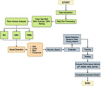
The methodology of this research consists of the following steps, as illustrated in Figure 1:
Figure 1. Research methodology flowchart
· Data acquisition and preprocessing. · Splitting data into training (80%) and testing (20%) subsets. · Analyzing the time horizon with options set at4, 24, and 120 hours. · Selecting models: CNN, LSTM, RNN, and Transformer architectures. · Applying a random search for optimal hyperparameter selection. · Evaluating models using the best metrics from tests. · Training the selected models with the best hyperparameters. |
|
· Testing the trained models. · Evaluating model performance using R2, RMSE, MAE, and MAPE. · Comparing results across models. · Drawing conclusions based on the model comparison and overall analysis.
2.2.Study case
The time series data used in this study were obtained from a weather station in Cuenca, Azuay, Ecuador, located at 7-77 Bolivar Street and Borrero Street (coordinates: latitude -2.897, longitude -79.00). Managed by the Empresa Municipal de Movilidad, Tránsito de Transporte de la Municipalidad de Cuenca (EMOVEP), this station provides publicly available data for personal, research, and governmental use. Positioned in a central area characterized by its commercial, tourist, colonial, and residential significance, this station is part of a network of three monitoring stations in Cuenca, as depicted in Figure 2.
Figure 2. EMOV-EP weather stations
2.3.Data preprocessing
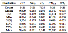
The meteorological station recorded gas emissions, including CO,NO2,O3, PM2.5, and SO2, at 10-minute intervals throughout 2022, generating approximately 52,560 records. These were exported in CSV format from the official EMOV-EP website. Where necessary, measurement units for pollutants were converted (e.g., CO from mg/m3 to ppm) to facilitate AQI calculation. Hourly averages were computed, reducing the dataset to 8,760 records. After filtering out null values and irrelevant data, 7,425 records were retained for analysis. Table 1 provides an overview of the time series data, while Figure 3 illustrates the hourly variation of the recorded gases. |
Table 1. Summary of the research time series
Figure 3. CO,NO2,O3, PM2.5, and SO2 registered per hour
Using the filtered values, the AQI for each pollutant was calculated following the guidelines outlined in the air quality report published by the U.S. Environmental Protection Agency [28]. The AQI computation is based on the pollutant concentration and is determined using Equation (1).
Where:
· IP is the contaminant index p. · CP is the rounded concentration of the pollutant p. · BPHI is the cut-off point that is greater than or equal to CP. · BPLO is the cutoff point that is less than or equal to CP. · IHI is the AQI value corresponding to BPHI. · ILO is the AQI value corresponding to BPLO.
|
|
The individual contaminant index values (Ip) for each pollutant p are calculated independently, and the final AQI is determined by selecting the maximum value from the set of calculated indices. This selection methodology ensures that the final AQI reflects the pollutant exhibiting the highest potential for adverse health impacts, providing a comprehensive assessment of air quality conditions. To analyze the relationship between the pollutants and the calculated AQI, a correlation matrix was constructed, as illustrated in Figure 4. Figure 4 illustrates that, in this specific case, based solely on the pollutant data recorded by the meteorological station, the AQI value exhibits a stronger correlation with CO and NO2, while its correlation with O3, PM2.5 and SO2 is minimal. This information will be considered for the development and configuration of the AI models in subsequent analyses.
Figure 4. Correlation matrix of the different pollutants
Standardization involves transforming the data such that it has a mean of 0 and a standard deviation of 1. This process is analytically represented by Equation (2), which was utilized in this research:
Where:
· X: It is the required value to be normalized. · Mean: The arithmetic means of the distribution. · Standard deviation: Standard deviation of the distribution.
Finally, after standardizing the time series values, the dataset was partitioned, with 80% allocated for training and 20% reserved for testing. |
2.4.Sliding window
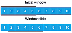
Hota, et al. [29] highlight that a commonly employed technique in time series analysis is the creation of sliding windows, which provides a temporal approximation of the true value of the time series data. This method accumulates historical time series data within a specified window to predict the subsequent value. Figure 5 illustrates the sliding window process with a window size of 5.
Figure 5. Sliding window process
Considering the aforementioned approach, sliding windows of 4, 24, and 120 hours were utilized to predict subsequent time intervals.
2.5.Deep learning
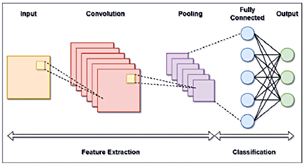
2.5.1. Convolutional Neural Networks (CNN), Recurrent Neural Networks (RNN), Long short-term memory (LSTM), Transformer model
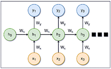
Recurrent Neural Networks (RNNs) are a class of neural networks specifically designed for processing sequential data. Their architecture enables the output of one layer to loop back into the input, allowing the network to retain memory of prior states. This capability makes RNNs particularly effective for tasks requiring contextual or historical information, including time series prediction, natural language processing, and speech recognition [30]. A standard RNN configuration is illustrated in Figure 7.
Figure 6. CNN standard configuration
|
|
Figure 7. RNN standard configuration
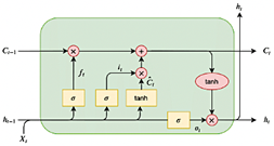
Long Short-Term Memory Networks (LSTMs) were developed to address the limitations of traditional RNNs, such as the vanishing gradient problem, by incorporating a memory cell capable of retaining information over extended periods [31]. Each LSTM cell comprises three gates: the input gate, which controls the incorporation of new information; the forget gate, which eliminates irrelevant data; and the output gate, which determines the information to be passed to the next step [31]. A standard LSTM configuration is depicted in Figure 8.
Figure 8. LSTM standard configuration [32]
Transformers have garnered considerable attention for their outstanding performance across various domains, including natural language processing (NLP), computer vision, and speech processing. Renowned for their ability to model long-term dependencies and complex interactions in sequential data, Transformers are particularly well-suited for time series prediction tasks [24]. The architecture implemented in this study is depicted in Figure 9.
Figure 9. Transformers model architecture. Adapted from Youness [33] |
2.6.Performance metrics
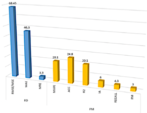
In the study conducted by Méndez, et al. [20], research aimed to identify the primary factors influencing air quality prediction during the period 2011–2021. The authors found that the most commonly applied metrics for evaluating machine learning (ML) models include RMSE, MAE, MAPE, ACC, and R2 as illustrated in Figure 10.
Figure 10. Evaluation of metrics usage [20]
2.6.1. Root mean square error (RMSE)
Root mean square error (RMSE) is a widely used metric that quantifies the average difference between predicted and observed values [34]. The formula for RMSE is presented in Equation (3):
Where: · n: number of samples. · yI : observed value. · yI : predicted value. · (yI −YI)2: squared error between predicted and observed values.
2.6.2. Mean absolute error (MAE)
Mean absolute error (MAE) is a metric used to assess the accuracy of a model by calculating the average of the absolute errors between predicted and observed values [34]. The formula for MAE is presented in Equation (4):
|
|
Where:
· n: number of samples. · yI : observed value. · yI : predicted value. · |yI − YI|: absolute error between predicted and observed values.
2.6.3. Mean absolute percentage error (MAPE)
Mean Absolute Percentage Error (MAPE) quantifies the average error as a percentage of the observed values, providing a scale-independent metric that facilitates comparisons across different models [34]. The formula for MAPE is presented in Equation (5):
Where:
· n: number of samples. · yI: observed value. · yI: predicted value. ·
2.6.4. Coefficient of determination (R2)
The coefficient of determination R2 quantifies the proportion of variance in the dependent variable that is explained by the independent variables of the model. An R2 value of 1 indicates that the model perfectly explains the variability in the data, whereas a value of 0 signifies that the model does not explain any variability [34]. The formula for R2 is presented in Equation (6):
Where:
· n: number of samples. · yI: observed value. · yI: predicted value. · y: mean of all observed values yI . ·
·
|
2.7.Random search
In ML, random search (RS) is an optimization technique used to identify optimal hyperparameters by exploring random combinations within a predefined parameter space. This approach is more efficient and computationally less expensive compared to exhaustive search methods [35]. Figure 11 illustrates the sequence of steps involved in the RS process.
Figure 11. Methodology of the random search technique
The process involves the following steps:
· Identifying the AI model to optimize and define its hyperparameters. · Setting ranges for each hyperparameter. · Specifying evaluation metrics, such as R2, MAE, and RMSE. · Randomly selecting combinations of hyperparameters. · Training the model and evaluating its performance. · Choosing the best-performing combination and retraining the model. · Validating the performance of the optimized model.
3. Results and discussion 3.1.Correlation Analysis
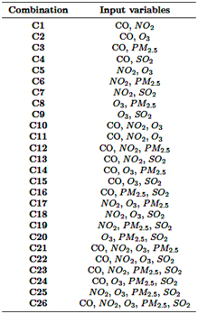
Figure 4 illustrates the relationship between variables using Pearson’s Correlation Coefficient to assess their correlation with maximum AQI concentration (AQIMAX). The heatmap reveals that CO has the strongest positive correlation with AQIMAX (0.56), followed by NO2 (0.3) and SO2 (0.16), while O3 shows a negative correlation (-0.36). Furthermore, CO is moderately correlated with NO2 (0.36) and SO2 (0.15), while O3 demonstrates inverse correlations with both CO (-0.41) and NO2 (-0.42). PM2.5 exhibits weak negative correlations with AQIMAX, CO, and NO2 These results highlight CO as the variable most strongly correlated with AQIMAX, providing critical guidance for selecting the input combinations outlined in Table 2. |
|
Table 2. Combinations of input variables
3.2.Results of the AI models
This section analyzes the performance outcomes of each model, considering the input combinations outlined in Table 3, the type of AI model employed, and the associated evaluation metrics.
Table 3. CNN model results
|
3.2.1. CNN results
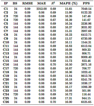
The CNN model was evaluated using 26 different input parameter combinations, all based on a 24-hour sliding window (Table 4). The R2 ranged from 0.620 to 0.698, with the combination of CO, O3, PM2.5, and SO2 (Row 24) achieving the highest performance at an R2 value of 0.698. Conversely, the combination involving NO2 and SO2 (Row 7) yielded the lowest performance, with an R2 of 0.620. Regarding error metrics, the RMSE ranged from 0.087 to 0.097, while the MAE varied from 0.060 to 0.068. Notably, the combination of CO, O3, PM2.5, and SO2 also exhibited the lowest errors, further highlighting its superior performance.
Table 4. RNN model results
The MAPE values, indicating prediction accuracy, ranged from15.48% to 18.83%. Combinations involving CO and O3 exhibited the lowest MAPE values, reflecting higher prediction accuracy. Conversely, combinations including NO2 and PM2.5 had higher MAPE values, indicating lower prediction accuracy. Computational efficiency varied significantly, with predictions rates ranging from 35,805 to 79,091 predictions per second. More complex combinations, such as CO, NO2, O3, PM2.5, and SO2 (Row 26), required up to 4.5 GB of RAM, yet achieved superior prediction rates. |
|
In summary, the combination of CO, O3, PM2.5, and SO2 (Row 24) emerged as the most accurate, achieving the highest R2, the lowest errors, and strong computational efficiency. In contrast, combinations including NO2 and SO2 underperformed across all metrics, suggesting these variables have a lesser impact on prediction accuracy. Where
· IP: Input Parameters · BS: Best Window · PPS: Predictions Per Second
3.2.2. RNN results
The RNN model was evaluated using 26 different combinations of input parameters within a 24-hour sliding window (Table 5). The R2 values ranged from 0.533 to 0.576, with the combination of CO, NO2, O3, and PM2.5 (Row 21) achieving the highest R2 of 0.576. Conversely, the combination involving NO2 and SO2 (Row 7) showed the lowest performance, with an R2 of 0.533. The RMSE values ranged from 0.092 to 0.097, while the MAE ranged from 0.058 to 0.063, with the combination of CO, NO2, O3, and PM2.5, demonstrating the lowest error rates, indicating superior performance.
Table 5. LSTM model results
The MAPE values ranged between 20.48% and 22.92%, with the lowest values observed in combinations that included CO and PM2.5, suggesting better prediction accuracy. In contrast, combinations involving NO2 and O3 exhibited higher MAPE values, indicating lower |
accuracy. Computational efficiency varied significantly, with prediction rates spanning 20,478 to 43,654 predictions per second. More complex combinations, such as CO, NO2, O3, PM2.5, and SO2 (Row 26), required up to 23.4 GB of RAM but demonstrated higher prediction throughput. In conclusion, the combination of CO, NO2, O3, and PM2.5 emerged as the most accurate, achieving the highest R2, the lowest error metrics, and strong computational efficiency. In contrast, combinations including NO2 and SO2 consistently underperformed across all metrics, suggesting these variables have a limited impact on prediction accuracy.
3.2.3. LSTM results
The LSTM model was evaluated using 26 different combinations of input parameters, primarily with a 24-hour sliding window, although some configurations employed 144-hour or 720-hour windows (Table 6). The R2 values ranged from 0.669 to 0.701, with the combination of CO, NO2, PM2.5, and SO2 (Row 23) achieving the highest R2 of 0.701. Conversely, the combination of NO2, O3, and SO2 (Row 18) exhibited the lowest R2 at 0.669. The RMSE values varied between 0.087 and 0.092, while the MAE ranged from 0.056 to 0.062, with the combination of CO, NO2, PM2.5, and SO2 demonstrating the lowest error metrics, signifying superior performance.
Table 6. Transformers model results
|
|
The MAPE values ranged from 15.31% to 17.31%, with the lowest values observed in combinations including CO and NO2, indicating superior prediction accuracy. Conversely, combinations involving NO2 and PM2.5 exhibited higher MAPE values, suggesting lower accuracy. Computational efficiency varied significantly, with predictions per second ranging from 116 to 8,613. Shorter sliding windows generally resulted in higher prediction rates but required increased RAM usage. For instance, complex combinations such as CO, NO2, O3, PM2.5, and SO2 (Row 26) demanded up to 4.4 GB of RAM and achieved moderate prediction rates. In contrast, simpler combinations like CO and NO2 required less RAM (3.3 GB) but exhibited lower prediction rates. In summary, the combination of CO, NO2, PM2.5, and SO2 (Row 23) emerged as the most accurate, achieving the highest R2 and the error metrics, albeit with increased computational demands. Conversely, combinations involving NO2 and SO2 exhibited consistently lower performance across all evaluated metrics.
3.2.4. Transformer results
In terms of error metrics, the RMSE ranged from 0.094 to 0.130, and the MAE from 0.068 to 0.099, with the lowest errors observed for the combination of CO, NO2, PM2.5, and SO2. Higher errors, particularly in MAE, were noted for combinations involving CO and SO2, suggesting these inputs are less effective for accurate predictions. The MAPE values varied between 18.19% and 26.83%, with the lowest values associated with combinations involving O3 and PM2.5, while higher MAPE values were observed for combinations including CO and O3 (Row 2). Regarding computational efficiency, predictions per second ranged from 2,974 to 21,030. More complex combinations with a greater number of input parameters and longer sliding windows required higher RAM usage (up to 3.7 GB) but achieved faster prediction rates. Conversely, simpler combinations, such as CO and NO2 required less RAM (1.8 GB) but exhibited slower prediction rates. Overall, the combination of CO, NO2, PM2.5, and SO2 (Row 23) emerged as the most accurate, achieving the highest R2 and the lowest error metrics, albeit with increased computational requirements. In contrast, combinations involving NO2 and O3 showed inferior performance across all metrics.
3.2.5. AI model results analysis
When comparing the performance of the RNN, CNN, LSTM, and Transformer models, the Transformer model |
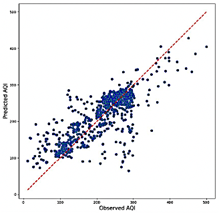
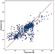
exhibits notably lower accuracy, with R2 values ranging from 0.322 to 0.640. This broad range underscores significant challenges in capturing the variability of the output data, particularly when utilizing variables such as NO2 and O3.While the Transformer model demonstrates higher computational efficiency—requiring 1.8 GB to 3.7 GB of RAM and achieving prediction rates between 2,974 and 21,030 predictions per second—this efficiency does not offset its lower predictive accuracy. As illustrated in Figure 12, the scatter plots for the Transformer model reveal substantial dispersion around the reference line, particularly at extreme AQI values. This deviation highlights the model’s unreliability in these situations.
Figure 12. Transformer model predictions combination 23 (Best R2 and RMSE)
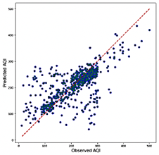
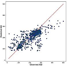
The RNN model, while more accurate than the Transformer, demonstrates intermediate performance with R2 values ranging from 0.533 to 0.576. The RNN achieves acceptable accuracy, with RMSE values between 0.092 and 0.097 and MAE values ranging from 0.058 to 0.063. However, its MAPE values, which fall between 20.48% and 22.92%, are higher than those observed for the CNN and LSTM models. As depicted in Figure 13, the RNN scatter plots exhibit a higher density of points near the y = x line compared to the Transformer model, suggesting improved overall alignment with observed values. Nonetheless, significant dispersion persists at the extreme AQI levels, highlighting variability in accuracy when predicting high or low AQI values.
Figure 13. Transformer model predictions combination 10 (Average R2) |
|
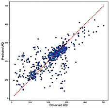
In terms of computational efficiency, the RNN exhibits a balanced performance, with RAM usage ranging from 22.8 GB to 23.4 GB and prediction rates between 20,478 and 43,654 predictions per second. While not exceptional, this performance positions the RNN as a viable option, offering a reasonable trade-off between accuracy and efficiency. The CNN model exhibited a higher R2 range of 0.620 to 0.698, demonstrating its strong capability to capture data variability and provide accurate predictions. Among the tested combinations, CO, O3, PM2.5, and SO2 yielded the best performance. The errors were relatively low, with RMSE values between 0.087 and 0.097 and MAE values ranging from 0.060 to 0.068. Additionally, MAPE values between 15.31% and 18.83% further underscored the model’s predictive accuracy. As illustrated in Figure 14, the scatter plots reveal the CNN model’s ability to deliver consistent predictions, with a significant clustering of data points around the regression line, even at extreme values, thereby minimizing errors. Although the CNN model is less computationally efficient than the Transformer, it maintains a reasonable balance, with RAM usage ranging from 3.8 GB to 4.5 GB and a prediction rate of 35,805 to 79,091 predictions per second.
Figure 14. Transformer model predictions combination 5 (Worst R2)
The LSTM model demonstrates superior accuracy among the evaluated models, with an R2 range of 0.669 to 0.701, highlighting its exceptional ability to discern patterns within the data. It outperforms other models in error metrics, achieving RMSE values between 0.087 and 0.092 and MAE values ranging from 0.056 to 0.062. Additionally, the LSTM model exhibits the lowest MAPE values, ranging |
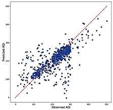
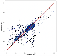
from 15.31% to 17.31%, underscoring its remarkable prediction accuracy. As illustrated in Figure 15, the scatter plots for the LSTM model reveal a high concentration of data points near the reference line, with minimal scatter, even for extreme AQI values. This consistency and precision position the LSTM as a robust and reliable option for applications where accuracy is critical. However, the LSTM model is the least computationally efficient among those evaluated, with RAM usage ranging from 3.3 GB to 4.5 GB and prediction speeds between 116 and 8,613 predictions per second. This relative inefficiency, especially when using longer sliding windows, may limit its applicability in scenarios where processing speed is critical. Nonetheless, its exceptional accuracy establishes it as a highly reliable option for applications where precision takes precedence over computational efficiency.
Figure 15. RNN model predictions combination 21 (Best R2)
Figure 16. RNN model predictions combination 20 (Average R2) |
|
Figure 17. RNN model predictions combination 7 (Worst R2)
Figure 18. CNN model prediction combination 24 (Best R2)
Figure 19. CNN model prediction combination 18 (Average R2)
|
Figure 20. CNN model prediction combination 7 (Worst R2)
Figure 21. LSTM model prediction combination 23 (Best R2)
Figure 22. LSTM model prediction combination 9 (Best R2) |
|
Figure 23. LSTM model prediction combination 14 (Average R2)
Figure 24. LSTM model prediction combination 18 (Worst R2)
3.2.6. Comparison with related studies
This study evaluates the effectiveness of LSTM, GRU, RNN, CNN and Transformer models for predicting the Air Quality Index (AQI) in Cuenca, Ecuador, and compares the results with findings from other relevant research, such as the study conducted by Cui et al. [36], which focused on PM2.5 prediction using Transformer and CNN-LSTM-Attention models in Beijing, China. A key distinction between the studies lies in the datasets and their characteristics. This study utilizes data from a single meteorological station in Cuenca, comprising 7,425 records for the year 2022. In contrast, the Beijing study employs data from 12 monitoring stations collected over four years (2013–2017), totaling over 35,000 records. The richer dataset in Beijing allowed researchers to incorporate seasonal variations and long-term dependencies, critical factors for accurate PM2.5 prediction. Additionally, their Transformer model was enhanced with multi-head attention mechanisms and positional encoding, enabling more effective capture of complex temporal patterns and seasonal fluctuations [36]. |
Regarding model performance, this study demonstrates that the LSTM model achieves the highest accuracy for AQI prediction in Cuenca, with an R2 of 0.701, surpassing the Transformer model’s performance, which achieved an approximate R2 of 0.68. Conversely, in the Beijing study, the Transformer model significantly outperformed the CNN-LSTM-Attention architecture, achieving an R2 of 0.944 compared to 0.836. This superior performance was attributed to the Transformer’s capacity to handle both abrupt meteorological changes and long-term trends, particularly during complex seasonal transitions such as those observed in autumn and winter [36]. Another notable difference is the prediction horizon. This study evaluated short- to medium-term prediction windows (4, 24, and 120 hours), whereas the Beijing study focused on hourly predictions. The Transformer model in Beijing proved particularly effective in capturing sudden pollutant variations driven by meteorological changes, underscoring its suitability for highfrequency predictions in dynamic environments [36]. These findings underscore the necessity of tailoring AI architectures to the unique characteristics of specific datasets and prediction objectives. Future research should focus on developing hybrid models that leverage the complementary strengths of LSTM and Transformer architectures, aiming to effectively tackle both local and regional air quality forecasting challenges.
4. Conclusions
In this study, the performance of various artificial intelligence models, including RNN, CNN, LSTM, and Transformers, was evaluated and compared for the task of predicting the Air Quality Index (AQI). The findings reveal that the LSTM model consistently outperformed the other models, achieving an R2 of 0.701 and an RMSE of 0.087. Its superior performance was particularly evident when using variable combinations such as CO, NO2, PM2.5, and SO2.The analysis underscores the LSTM model’s effectiveness in capturing complex temporal relationships among these variables, establishing it as a reliable and valuable tool for accurate AQI prediction in diverse scenarios. Although Transformers models have demonstrated exceptional performance in various fields such as natural language processing (NLP) and computer vision (CV), their application to AQI prediction, particularly with this specific dataset, reveals significant limitations. In this study, Transformers exhibited notable variability in performance, with coefficients of determination ranging from 0.322 to 0.640. These findings suggest that Transformers face challenges in effectively capturing the intrinsic complexity of the analyzed time-series data, |
|
particularly when using variable combinations that include NO2 and O3. Despite their computational efficiency, the predictive accuracy of Transformers for AQI falls short compared to more competitive models such as LSTM. In terms of computational efficiency, both CNN and LSTM models have demonstrated their suitability for real-time applications, offering an effective balance between accuracy and resource utilization. The LSTM model, in particular, stands out for its exceptional predictive accuracy, efficient RAM usage of approximately 4.4 GB, and its capability to perform a substantial number of predictions per second. This combination of high performance and resource efficiency makes LSTM especially well-suited for air quality prediction systems that require fast and precise responses, such as real-time environmental monitoring applications. Despite achieving satisfactory R2 values, the analysis revealed considerable data dispersion and elevated error metrics across all implementations, rendering some models unsuitable for reliable deployment. This study serves as a comparative evaluation of artificial intelligence approaches, highlighting both the strengths and limitations of current AI architectures for AQI forecasting. The findings underscore the need for refinement in existing implementations while emphasizing the substantial potential of AI models for improving air quality predictions in the future. In conclusion, the training of all models encountered limitations due to the relatively small size of the Cuenca dataset and the low correlation observed between certain pollutants. For future research, we recommend leveraging larger datasets and extending the analysis over longer periods to enhance model performance and generate more robust insights.
4.1.Future directions
The selection of Long Short-Term Memory (LSTM), Convolutional Neural Networks (CNN), Transformer, and Recurrent Neural Networks (RNN) architectures as foundational models in this study was based on their established prominence in time series analysis and their significant contributions to advancements in AI research. Building upon these foundational architectures, future research should explore the incorporation of enhanced Transformer-based models through the integration of multi-head attention mechanisms and positional encoding schemes. These enhancements could enable more sophisticated modeling of temporal dependencies in air quality patterns. The implementation of Physics-Informed Neural Networks (PINNs) also presents a promising direction, as these architectures explicitly integrate |
fundamental atmospheric physics and chemical transport equations into the neural network framework. This approach offers the potential to bridge the gap between data-driven methodologies and theoretical models, enhancing the interpretability and accuracy of predictions. While established architectures such as Transformers, CNNs, RNNs, and LSTMs have demonstrated notable efficacy, exploring emerging methodologies like Neural Ordinary Differential Equations (Neural ODEs), Temporal Fusion Transformers, and Informer networks could yield even greater predictive capabilities. These novel approaches, though less widely adopted in AI research, may address existing challenges in modeling non-linear atmospheric dynamics and complex inter-variable correlations, thus advancing AQI forecasting to new levels of precision and reliability.
References
[1] J. Zhang and S. Li, “Air quality index forecast in beijing based on cnnlstm multi-model,” Chemosphere, vol. 308, p. 136180, 2022. [Online]. Available: https://doi.org/10.1016/j.chemosphere.2022.136180 [2] M. Ansari and M. Alam, “An intelligent iotcloud- based air pollution forecasting model using univariate time-series analysis,” Arabian Journal for Science and Engineering, vol. 49, no. 3, pp. 3135–3162, Mar 2024. [Online]. Available: https://doi.org/10.1007/s13369-023-07876-9 [3] F. Cassano, A. Casale, P. Regina, L. Spadafina, and P. Sekulic, “A recurrent neural network approach to improve the air quality index prediction,” in Ambient Intelligence – Software and Applications –,10th International Symposium on Ambient Intelligence, P. Novais, J. Lloret, P. Chamoso, D. Carneiro, E. Navarro, and S. Omatu, Eds. Cham: Springer International Publishing, 2020, pp. 36–44. [Online]. Available: https://doi.org/10.1007/978-3-030-24097-4_5 [4] K. Oguz and M. A. Pekin, Prediction of Air Pollution with Machine Learning Algorithms. 1–12: Turkish Journal of Science and Technology, 2024, vol. 19, no. 1. [Online]. Available: https://doi.org/10.55525/tjst.1224661 [5] H. Jalali, F. Keynia, F. Amirteimoury, and A. Heydari, “A short-term air pollutant concentration forecasting method based on a hybrid neural network and metaheuristic optimization algorithms,” Sustainability, vol. 16, no. 11, 2024. [Online]. Available: https://doi.org/10.3390/su16114829 |
|
[6] R. Patil, D. Dinde, and S. Powar, “A literature review on prediction of air quality index and forecasting ambient air pollutants using machine learning algorithms,” International Journal of Innovative Science and Research Technology, vol. 5, pp. 1148–1152, 09 2020. [Online]. Available: http://dx.doi.org/10.38124/IJISRT20AUG683 [7] R. Hassan, M. Rahman, and A. Hamdan, “Assessment of air quality index (aqi) in riyadh, saudi arabia,” IOP Conference Series: Earth and Environmental Science, vol. 1026, no. 1, p. 012003, may 2022. [Online]. Available: https://dx.doi.org/10.1088/1755-1315/1026/1/012003 [8] W.-T. Tsai and Y.-Q. Lin, “Trend analysis of air quality index (aqi) and greenhouse gas (ghg) emissions in taiwan and their regulatory countermeasures,” Environments, vol. 8, no. 4, 2021. [Online]. Available: https://doi.org/10.3390/environments8040029 [9] G. Ravindiran, S. Rajamanickam, K. Kanagarathinam, G. Hayder, G. Janardhan, P. Arunkumar, S. Arunachalam, A. A. AlObaid, I. Warad, and S. K. Muniasamy, “Impact of air pollutants on climate change and prediction of air quality index using machine learning models,” Environmental Research, vol. 239, p. 117354, 2023. [Online]. Available: https://doi.org/10.1016/j.envres.2023.117354 [10] N. P. Canh, W. Hao, and U. Wongchoti, “The impact of economic and financial activities on air quality: a chinese city perspective,” Environmental Science and Pollution Research, vol. 28, no. 7, pp. 8662–8680, Feb 2021. [Online]. Available: https://doi.org/10.1007/s11356-020-11227-8 [11] T. Madan, S. Sagar, and D. Virmani, “Air quality prediction using machine learning algorithms –a review,” in 2020 2nd International Conference on Advances in Computing, Communication Control and Networking (ICACCCN), 2020, pp. 140–145. [Online]. Available: https://doi.org/10.1109/ICACCCN51052.2020.9362912 [12] M. Kaur, D. Singh, M. Y. Jabarulla, V. Kumar, J. Kang, and H.-N. Lee, “Computational deep air quality prediction techniques: a systematic review,” Artificial Intelligence Review, vol. 56, no. 2, pp. 2053–2098, Nov 2023. [Online]. Available: https://doi.org/10.1007/s10462-023-10570-9 |
[13] S. Senthivel and M. Chidambaranathan, “Machine learning approaches used for air quality forecast: A review,” Revue d’Intelligence Artificielle, vol. 36, no. 1, pp. 73–78, 2022. [Online]. Available: https://doi.org/10.18280/ria.360108 [14] Q. Wu and H. Lin, “A novel optimalhybrid model for daily air quality index prediction considering air pollutant factors,” Science of The Total Environment, vol 683, pp. 808–821, 2019. [Online]. Available: https://doi.org/10.1016/j.scitotenv.2019.05.288 [15] Y. Xu, H. Liu, and Z. Duan, “A novel hybrid model for multi-step daily aqi forecasting driven by air pollution big data,” Air Quality, Atmosphere & Health, vol. 13, no. 2, pp. 197–207, Feb 2020. [Online]. Available: https://doi.org/10.1007/s11869-020-00795-w [16] Z. Zhao, J. Wu, F. Cai, S. Zhang, and Y.-G. Wang, “A statistical learning framework for spatial-temporal feature selection and application to air quality index forecasting,” Ecological Indicators, vol. 144, p. 109416, 2022. [Online]. Available: https://doi.org/10.1016/j.ecolind.2022.109416 [17] J. A. Moscoso-López, D. Urda, J. González- Enrique, J. J. Ruiz-Aguilar, and I. Turias, “Hourly air quality index (aqi) forecasting using machine learning methods,” in 15th International Conference on Soft Computing Models in Industrial and Environmental Applications (SOCO 2020), 2021, pp. 123–132. [Online]. Available: https://upsalesiana.ec/ing33ar6r17 [18] B. S. Chandar, P. Rajagopalan, and P. Ranganathan, “Short-term aqi forecasts using machine/ deep learning models for san francisco, ca,” in 2023 IEEE 13th Annual Computing and Communication Workshop and Conference (CCWC), 2023, pp. 0402–0411. [Online]. Available: https://doi.org/10.1109/CCWC57344.2023.10099064 [19] J. Wang, P. Du, Y. Hao, X. Ma, T. Niu, and W. Yang, “An innovative hybrid model based on outlier detection and correction algorithm and heuristic intelligent optimization algorithm for daily air quality index forecasting,” Journal of Environmental Management, vol. 255, p. 109855, 2020. [Online]. Available: https://doi.org/10.1016/j.jenvman.2019.109855 [20] M. Méndez, M. G. Merayo, and M. Núñez, “Machine learning algorithms to forecast air quality: a survey,” Artificial Intelligence Review, vol. 56, no. 9, pp. 10 031–10 066, Sep 2023. [Online]. Available: https://doi.org/10.1007/s10462-023-10424-4 |
|
[21] C. Ji, C. Zhang, L. Hua, H. Ma, M. S. Nazir, and T. Peng, “A multi-scale evolutionary deep learning model based on ceemdan, improved whale optimization algorithm, regularized extreme learning machine and lstm for aqi prediction,” Environmental Research, vol. 215, p. 114228, 2022. [Online]. Available: https://doi.org/10.1016/j.envres.2022.114228 [22] R. Yan, J. Liao, J. Yang, W. Sun, M. Nong, and F. Li, “Multi-hour and multi-site air quality index forecasting in beijing using cnn, lstm, cnn-lstm, and spatiotemporal clustering,” Expert Systems with Applications, vol. 169, p. 114513, 2021. [Online]. Available: https://doi.org/10.1016/j.eswa.2020.114513 [23] E. Hossain, M. A. U. Shariff, M. S. Hossain, and K. Andersson, “A novel deep learning approach to predict air quality index,” in Proceedings of International Conference on Trends in Computational and Cognitive Engineering, M. S. Kaiser, A. Bandyopadhyay, M. Mahmud, and K. Ray, Eds. Singapore: Springer Singapore, 2021, pp. 367–381. [Online]. Available: https://doi.org/10.1007/978-981-33-4673-4_29 [24] Q. Wen, T. Zhou, C. Zhang, W. Chen, Z. Ma, J. Yan, and L. Sun, “Transformers in time series: a survey,” in Proceedings of the Thirty-Second International Joint Conference on Artificial Intelligence, ser. IJCAI ’23, Macao, P.R.China, 2023. [Online]. Available: https://doi.org/10.24963/ijcai.2023/759 [25] Y. Guo, T. Zhu, Z. Li, and C. Ni, “Auto-modal: Air-quality index forecasting with modal decomposition attention,” Sensors, vol. 22, no. 18, 2022. [Online]. Available: https://doi.org/10.3390/s22186953 [26] S. Ma, J. He, J. He, Q. Feng, and Y. Bi, “Forecasting air quality index in yan’an using temporal encoded informer,” Expert Systems with Applications, vol. 255, p. 124868, 2024. [Online]. Available: https://doi.org/10.1016/j.eswa.2024.124868 [27] J. Xie, J. Li, M. Zhu, and Q. Wang, “Multi-step air quality index forecasting based on parallel multi-input transformers,” in Pattern Recognition, H. Lu, M. Blumenstein, S.-B. Cho, C.-L. Liu, Y. Yagi, and T. Kamiya, Eds. Cham: Springer Nature Switzerland, 2023, pp. 52–63. [Online]. Available: https://doi.org/10.1007/978-3-031-47665-5_5 [28] U.S. Environmental Protection Agency, Guideline for Reporting of Daily Air Quality – Air Quality Index (AQI). U.S. Environmental Protection Agency Research Triangle Park, North Carolina, 2006. [Online]. Available: https://upsalesiana.ec/ing33ar6r28 |
[29] H. S. Hota, R. Handa, and A. K. Shrivas, “Time series data prediction using sliding window based rbf neural network,” in International Journal of Computational Intelligence Research, vol. 13, no. 5, 2017, pp. 1145–1156. [Online]. Available: https://upsalesiana.ec/ing33ar6r29 [30] D. C. Yadav and S. Pal, “15 - measure the superior functionality of machine intelligence in brain tumor disease prediction,” in Artificial Intelligence-Based Brain-Computer Interface, V. Bajaj and G. Sinha, Eds. Academic Press, 2022, pp. 353–368. [Online]. Available: https://doi.org/10.1016/B978-0-323-91197-9.00005-9 [31] A. Sherstinsky, “Fundamentals of recurrent neural network (rnn) and long short-term memory (lstm) network,” Physica D: Nonlinear Phenomena, vol. 404, p. 132306, 2020. [Online]. Available: https://doi.org/10.1016/j.physd.2019.132306 [32] S. Hesaraki. (2023) Long short-term memory (lstm). Medium. Human Stories ideas. [Online]. Available: https://upsalesiana.ec/ing33ar6r32 [33] Y. Mansar. (2021) How to use transformer networks to build a forecasting model. Medium. Human Stories ideas. [Online]. Available: https://upsalesiana.ec/ing33ar6r33 [34] J. A. Segovia, J. F. Toaquiza, J. R. Llanos, and D. R. Rivas, “Meteorological variables forecasting system using machine learning and open-source software,” Electronics, vol. 12, no. 4, 2023. [Online]. Available: https://doi.org/10.3390/electronics12041007 [35] M. Hammad Hasan. (2023) Tuning model hyperparameters with random searcha comparison with grid search. Medium. Human Stories ideas. [Online]. Available: https://upsalesiana.ec/ing33ar6r35 [36] B. Cui, M. Liu, S. Li, Z. Jin, Y. Zeng, and X. Lin, “Deep learning methods for atmospheric pm2.5 prediction: A comparative study of transformer and cnn-lstmattention,” Atmospheric Pollution Research, vol. 14, no. 9, p. 101833, 2023. [Online]. Available: https://doi.org/10.1016/j.apr.2023.101833 |
